Introduction

The Fourier Transform is pretty fundamental to digital signal processing (DSP). Some would go so far as to say it is the center of DSP, although I consider that a stretch. What was unclear to me was how it does what it does, and how I might somehow plumb its depths in a way that could transfer a deeper understanding of what was going on into my working model of software radios.

Before you read any further though I think it is probably a good idea to talk about who this article is for and who it is not for. This article is not for people who just use the function, specifically if you’re a MATLAB or Octave user and you understand all of this stuff from a pure math level, you probably won’t get a lot out of this article. If on the other hand you’ve got some basic math skills and you know how to write code and maybe you heard DSP was cool and want to understand it at a nuts and bolts level, well this could be a good resource for that.

In my case I had to take the necessary math and signal processing courses as part of my EE degree but frankly I felt this was all “analog” stuff that I would probably not use as I was a computer guy. So for me, it was kind of like trying to learn a foreign language where you took classes in it in college but you never used it in your day to day life so forgot most of what you knew anyway.

That said, the signal analyzer and “waterfall” displays are pretty slick and I love that they look very futuristic. As I started diving into SDR I found people would look at a spectrum analzer output and make some insightful comment about what was going on and I needed a fundamental understanding of what was going on if I wanted to have any chance of seeing those same insights.

I tend to learn by building things and manipulating things so that is where I started. I set out to build a set of functions and tools that would let me explore this space. This is something of a trip report of some steps of that journey.

Fourier’s Big Idea

Joseph Fourier was a brilliant mathematician that lived in France in the late 1700’s and early 1800’s. As part of an effort to understand heat flow in solids he pulled together earlier work and showed that any continuous waveform could be decomposed into a series of sinusoids.

Most texts go on to show how you can add sine waves together to make a square wave, a good example of this is on Wikipedia’s Fourier Transform Article. And in fact any closed form curve can be represented by a bunch of sine waves, even numbers and letters, what we’re interested in for SDR is being able to see what frequency components are in a signal at any given time. As such the question becomes how do you transform a signal in the time domain, which is to say one that could be plotted with time on the X axis, and amplitude on the Y axis like an oscilloscope does, into one plotted in the frequency domain, where frequency is on the X axis and amplitude is on the Y axis. This is the graphic that is plotted on most SDR displays, called a periodogram or spectrogram, to show you “the spectrum.”

I really wanted to know how it did that and so started exploring the Fourier transform and more importantly for me, its implementation. Fortunately, all of this math works at all frequencies, whether they are in the audio domain or the microwave region (where SDRs use it for filters and tuners). Much of the experimentation I’ve done has been at audio frequencies because it is something you can listen too and hear the differences.

A Note About Digitalness

When I started down this path I was operating under the assumption that a bunch of values for a sine wave were identical to the sine wave itself. Except that isn’t true, and the assumption lead me into some misunderstandings about what was going on.

The sine function is continuous over time. What that means is that for any arbitrarily small increment of time, you can compute the next value in the function. What is more, the difference in magnitude of the current value and the next value, its slope (and also the first derivative) tells what phase of the waveform you are in, from the first quadrant to the last.

When you break the waveform up into samples, you lose critical information about the waveform. Specifically you lose access to phase information that would let you unambiguously determine its frequency.

Sample FFT Plot

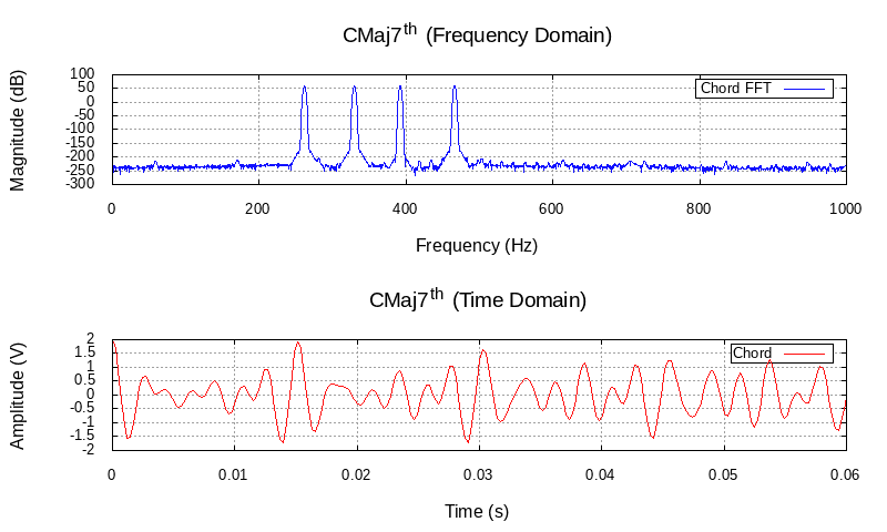
That should be a sample FFT plot. The magnitude is plotted in decibels dB.

Mixing and Correlation

Let’s get down to the basics. A the fourier transform of the C major chord is shown below.

The C Major 7th Chord